This workflow starts with complete Study Results and a long laboratory CSV. The laboratory file contains one row per participant and physical tube ID.
library(carwatch)

fixture <- system.file("extdata", "parity", "v1.0.0", package = "carwatch")
study_results <- read_study_results(file.path(fixture, "results.csv"))
saliva <- read_saliva(file.path(fixture, "saliva.csv"))

saliva
#> # A tibble: 2 × 3
#>   participant sample cortisol
#>   <chr>       <chr>     <dbl>
#> 1 VP01        tube-a        5
#> 2 VP01        tube-b        9
Merge laboratory values
Matching by sample uses the physical tube recorded by the app. This preserves the distinction between the tube planned for a position and the tube actually scanned there.
merged <- merge_saliva(study_results, saliva, match_on = "sample")
samples <- as_sample_events(merged)
samples[c(
  "participant", "day", "sample_position", "sample", "recorded_sample",
  "cortisol", "sample_compliant", "mismatch_corrected"
)]
#> # A tibble: 2 × 8
#>   participant day   sample_position sample recorded_sample cortisol
#>   <chr>       <chr>           <int> <chr>  <chr>              <dbl>
#> 1 VP01        D1                  1 tube-a tube-a                 5
#> 2 VP01        D1                  2 tube-b tube-b                 9
#> # ℹ 2 more variables: sample_compliant <lgl>, mismatch_corrected <lgl>
If a laboratory export identifies observations by day and sample
position, use match_on = "position" and provide the
day and sample_position columns instead.
Calculate response features
compute_features_from_carwatch() orders each curve by
registered sample position and uses the actual minutes since
awakening.
compute_features_from_carwatch(merged, saliva_type = "cortisol")
#> # A tibble: 1 × 14
#>   participant day   day_compliant expected_sample_count recorded_sample_count
#>   <chr>       <chr> <lgl>                         <int>                 <int>
#> 1 VP01        D1    TRUE                              2                     2
#> # ℹ 9 more variables: assessed_sample_count <int>,
#> #   compliant_sample_count <int>, non_compliant_samples <chr>,
#> #   cortisol_auc_g <dbl>, cortisol_auc_i <dbl>, cortisol_ini_val <dbl>,
#> #   cortisol_max_val <dbl>, cortisol_max_inc <dbl>, cortisol_slope12 <dbl>
Inspect timing and measurements
plot_sampling_timeline(merged, participant = "VP01", day = "D1")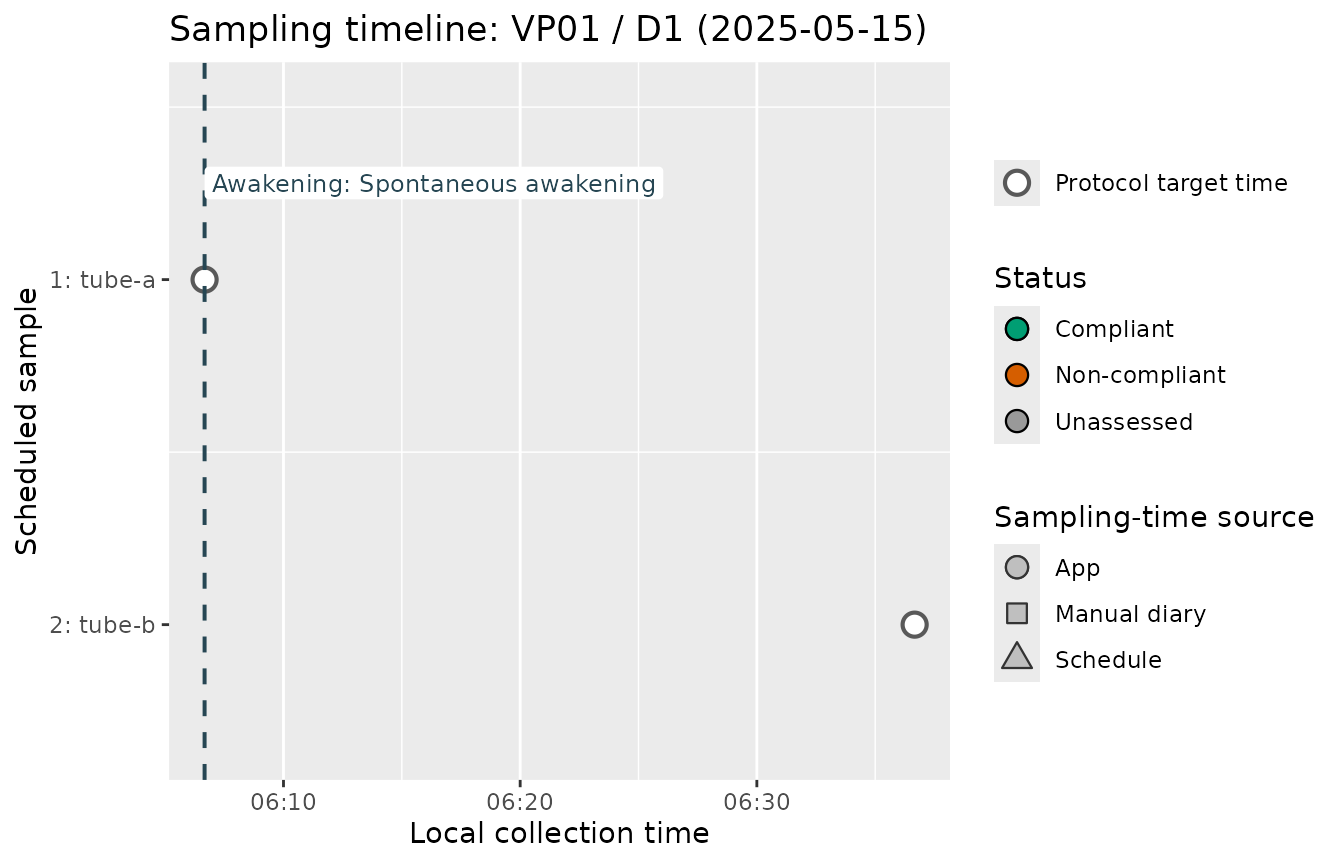
plot_compliance_overview(merged)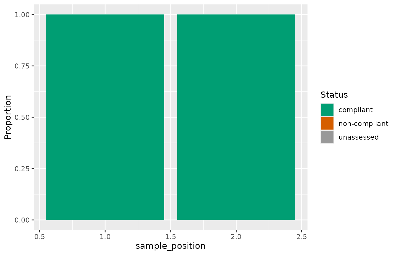
plot_timing_deviation(merged)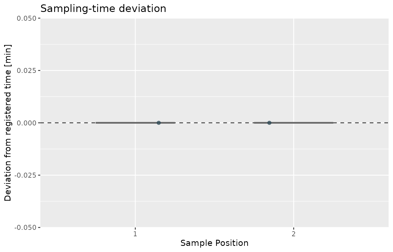
plot_saliva_curve(merged, value = "cortisol", ci = NULL)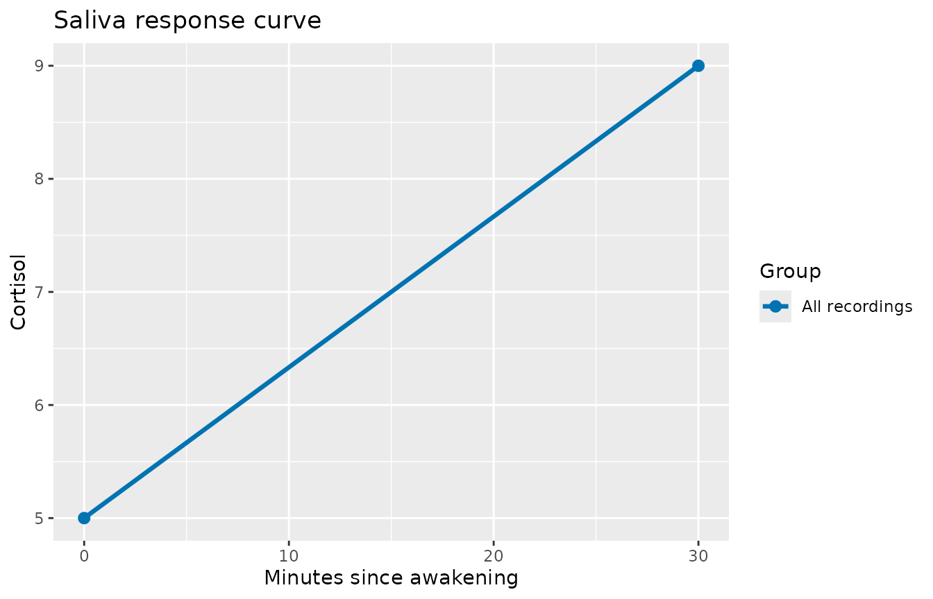
These plots return ordinary ggplot2 objects, so themes,
labels, and export settings can be adjusted with the normal
ggplot2 workflow.