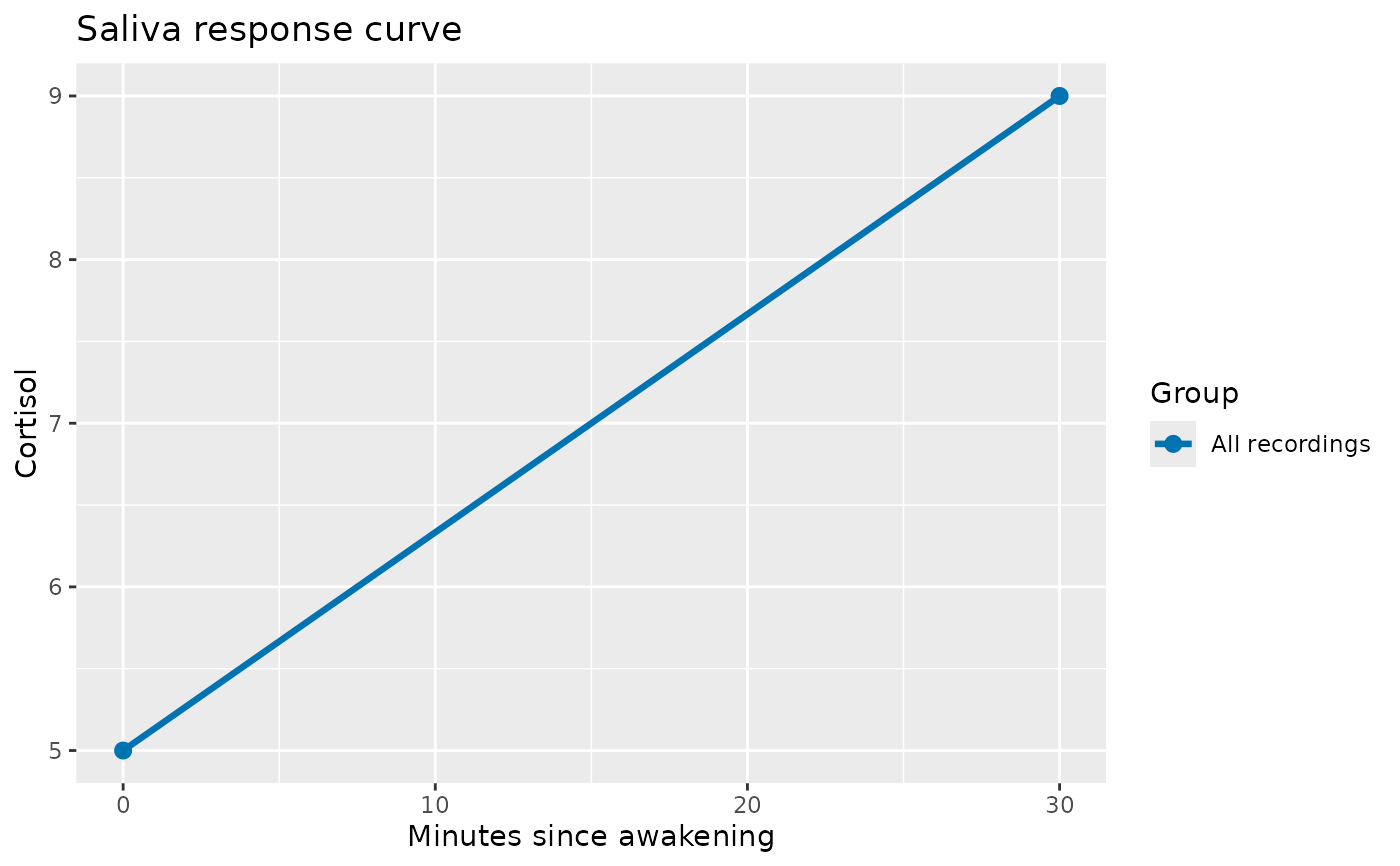
Plot CARWatch-aligned saliva response curves — plot_saliva

Actual time_min values define the horizontal axis. Faint lines show participant-day curves. Thick lines connect group means calculated separately at each registered sample_position; shaded ribbons show BCa bootstrap confidence intervals when at least two measurements contribute.

Usage

plot_saliva_curve(
  data,
  value = "cortisol",
  participant = NULL,
  day = NULL,
  group_by = NULL,
  ci = 95,
  n_boot = 1000,
  seed = 0,
  show_individual = TRUE
)

Arguments

data: Canonical results or sample events.
value: Non-empty name of the saliva measurement column.
participant: Optional exact participant filter.
day: Optional exact canonical-day filter.
group_by: Optional character vector defining separate aggregate curves.
ci: Bootstrap confidence level between 0 and 100, or NULL for no band.
n_boot: Positive number of bootstrap resamples.
seed: Integer random seed, or NULL to use the current R RNG state.
show_individual: Whether individual participant-day curves are drawn.

Value

A ggplot object.

Examples

fixture <- system.file("extdata", "parity", "v1.0.0", package = "carwatch")
results <- read_study_results(file.path(fixture, "results.csv"))
saliva <- read_saliva(file.path(fixture, "saliva.csv"))
merged <- merge_saliva(results, saliva)
plot_saliva_curve(merged, ci = NULL)